Graph Traversal on a Grid: Matrix Problems in Disguise

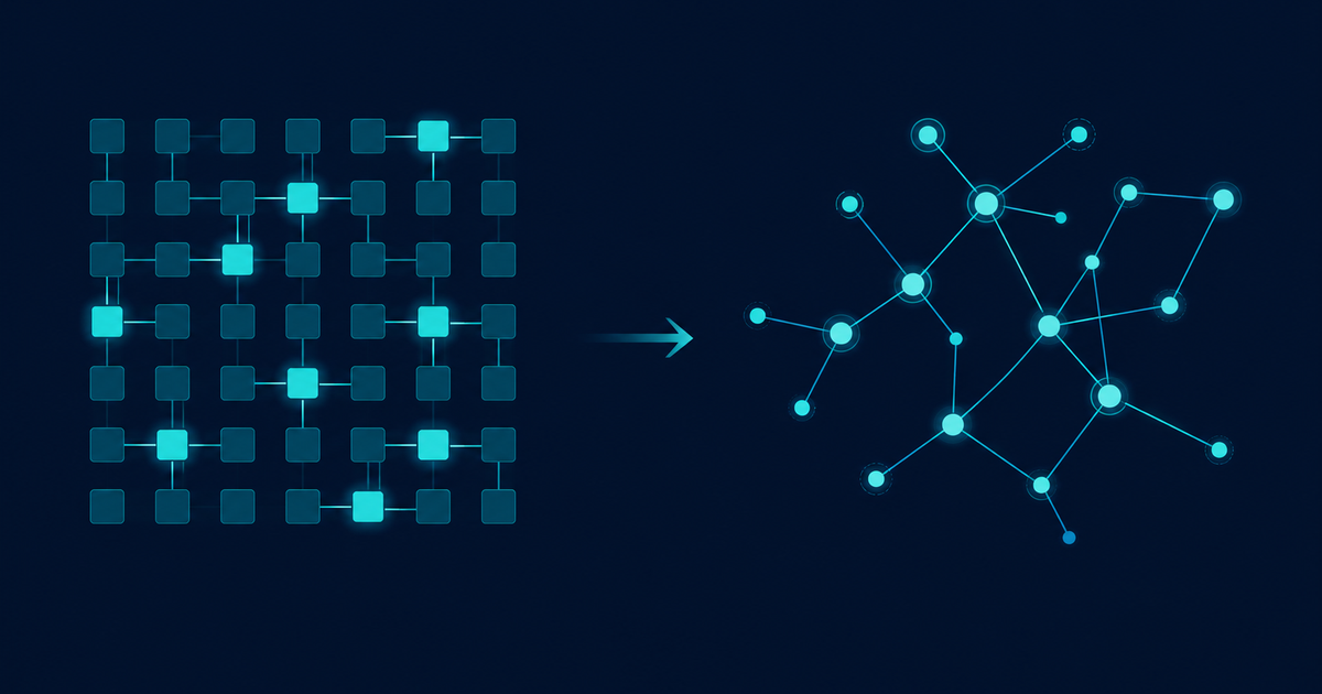
Most engineers who freeze on a grid question have already solved the same problem in another costume. They can write breadth first search on an adjacency list without hesitation, then stall completely when the input arrives as a two dimensional array of characters. The algorithm did not change, only the packaging did.

This is the single highest leverage pattern recognition skill in the coding interview, because grid questions are everywhere. Islands, rotting fruit, maze escapes, flood fill, word puzzles, shortest paths through obstacles: every one of them is graph traversal with the edges left implicit. Once you internalize the translation in both directions, a large chunk of the problem space collapses into one template you already know.

Every matrix is already a graph

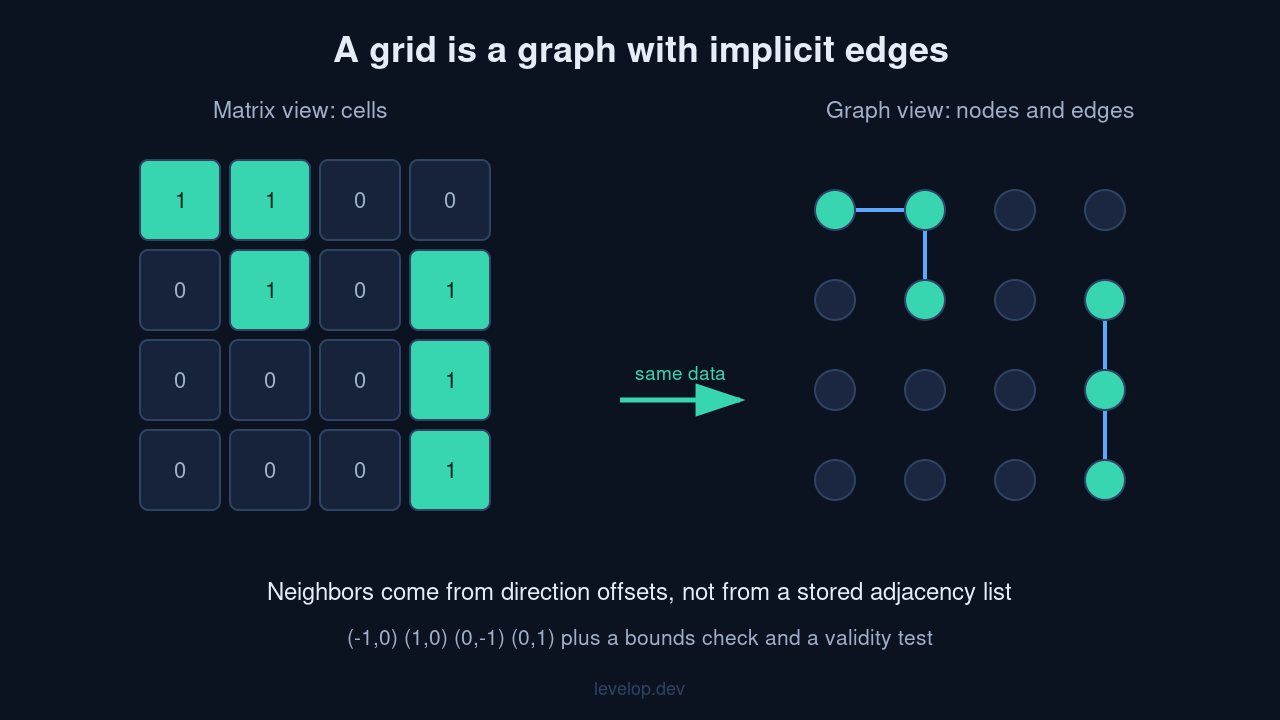
A graph is a set of nodes plus a rule for which nodes connect, and nothing in that definition requires you to store the edges. A grid satisfies both halves for free: each cell is a node, and the connection rule is arithmetic rather than lookup. Two cells are neighbors when their row and column differ by one step in an allowed direction.

That is the entire translation, and it explains why the standard adjacency lookup disappears in grid code. You are not reading edges out of memory, you are computing them on demand from a fixed list of direction offsets.

The implicit adjacency rule

For a four directional grid the neighbor rule is a fixed offset list, and a cell qualifies as a neighbor only if it stays inside the bounds and passes whatever validity test the problem defines.

DIRECTIONS = [(-1, 0), (1, 0), (0, -1), (0, 1)]

def neighbors(grid, r, c):
    rows, cols = len(grid), len(grid[0])
    for dr, dc in DIRECTIONS:
        nr, nc = r + dr, c + dc
        if 0 <= nr < rows and 0 <= nc < cols and grid[nr][nc] != '#':
            yield nr, nc

Swap those four offsets for the eight surrounding ones and you have a king move grid. Swap them for the eight knight offsets and you have a chessboard graph where adjacent means a legal knight jump, which is exactly how the classic minimum knight moves question is solved. The traversal code sitting above that neighbor function never changes at all.

Graph traversal when there are no edges to store

Once neighbors are a function rather than a data structure, the two core graph traversal algorithms drop straight in. Breadth first search explores in rings outward from the source, which is what makes it the correct tool for shortest path on an unweighted graph, while depth first search commits to one branch until it dead ends, which makes it the natural fit for connectivity, region shape, and backtracking questions.

from collections import deque

def bfs(grid, start):
    seen = {start}
    queue = deque([(start, 0)])
    while queue:
        (r, c), dist = queue.popleft()
        for nr, nc in neighbors(grid, r, c):
            if (nr, nc) not in seen:
                seen.add((nr, nc))
                queue.append(((nr, nc), dist + 1))
    return seen

The complexity argument is identical to the general case, because every cell enters the queue at most once and each of its constant number of neighbors is inspected once, so a grid with R rows and C columns costs linear time and linear space in the number of cells. Written the usual way as O(V + E), the grid simply has V equal to R times C and E bounded by four times that. If you want the deeper comparison of when each strategy applies, we broke that down in BFS vs DFS vs DP.

Four matrix problems that are graph traversal problems

Naming the underlying algorithm out loud before you write code is the habit that separates candidates who look fluent from candidates who look lucky, and these four translations cover most of what actually gets asked.

Counting islands is counting connected components

The question asks how many separate landmasses exist in a grid of land and water, and stripped of the theme it asks how many connected components a graph has. The standard algorithm is unchanged: iterate every node, and each time you find an unvisited one, launch a traversal that marks the entire component, then increment a counter.

def count_islands(grid):
    rows, cols = len(grid), len(grid[0])
    seen, count = set(), 0
    for r in range(rows):
        for c in range(cols):
            if grid[r][c] == '1' and (r, c) not in seen:
                count += 1
                stack = [(r, c)]
                seen.add((r, c))
                while stack:
                    cr, cc = stack.pop()
                    for nr, nc in neighbors(grid, cr, cc):
                        if grid[nr][nc] == '1' and (nr, nc) not in seen:
                            seen.add((nr, nc))
                            stack.append((nr, nc))
    return count

Note the explicit stack instead of recursion. On a grid of a thousand by a thousand cells a recursive depth first search can bury the interpreter under its own call stack, and that failure mode shows up in interviews often enough to be worth pre-empting.

Rotting oranges is multi source breadth first search

Fresh fruit spoils when it touches spoiled fruit, and you are asked for the number of minutes until nothing fresh remains. The instinct to run one search per rotten cell is what makes this feel hard, and it is also what makes it slow. The correct move is to seed the queue with every rotten cell at distance zero, which is equivalent to adding a virtual super source connected to all of them.

Multi source breadth first search is the most reusable variant in the whole family, and it generalizes far beyond fruit to nearest exit, distance to the closest zero, walls and gates, and fire spreading through a maze. We covered the stateful and bidirectional variants in advanced BFS patterns.

Word search is depth first search with backtracking

Here the traversal has to undo itself. You mark a cell as used while exploring a candidate path and unmark it when the path fails, because that cell may legitimately belong to a different path. This is the one grid pattern where breadth first search is a poor fit, since the state you care about is the path itself rather than the distance from a source.

def exists(grid, word):
    rows, cols = len(grid), len(grid[0])

    def dfs(r, c, i):
        if i == len(word):
            return True
        if not (0 <= r < rows and 0 <= c < cols) or grid[r][c] != word[i]:
            return False
        saved, grid[r][c] = grid[r][c], '#'
        found = any(dfs(r + dr, c + dc, i + 1) for dr, dc in DIRECTIONS)
        grid[r][c] = saved
        return found

    return any(dfs(r, c, 0) for r in range(rows) for c in range(cols))

Shortest path with obstacles is unweighted breadth first search

When every move costs the same, breadth first search is optimal and Dijkstra is overkill. Reach for a priority queue only when the moves carry different costs, for example when breaking a wall costs one and walking a corridor costs zero. That zero one weighting has its own specialized answer, the double ended queue variant known as 0-1 BFS, which pushes zero cost moves onto the front and unit cost moves onto the back.

The reverse translation: graph problems that want a matrix

The disguise runs the other way too, and this direction is the one most candidates never practice. Some genuine graph problems become dramatically simpler once you stop thinking in adjacency lists and store the graph as a two dimensional table instead.

When the adjacency matrix of a graph is the better representation

The adjacency matrix of a graph is a table where the entry at row i and column j records whether an edge runs from node i to node j. It costs quadratic space regardless of how few edges exist, which is why sparse graphs are usually stored as lists, but it buys you constant time edge lookup, and on a dense graph the memory penalty largely evaporates because the edge count approaches the square of the node count anyway.

Interview inputs frequently hand you the matrix form directly. Questions phrased as given an n by n grid where a one means city i and city j are linked, count the provinces, are connected components questions wearing a matrix costume, and the neighbor loop simply becomes a scan across one row.

def count_provinces(is_connected):
    n = len(is_connected)
    seen, count = set(), 0
    for start in range(n):
        if start in seen:
            continue
        count += 1
        stack = [start]
        seen.add(start)
        while stack:
            node = stack.pop()
            for other in range(n):
                if is_connected[node][other] and other not in seen:
                    seen.add(other)
                    stack.append(other)
    return count

All pairs shortest paths belongs in a table

Floyd-Warshall computes the shortest distance between every pair of nodes by relaxing paths through one intermediate node at a time, and it is essentially three nested loops over a distance matrix. On a graph small enough that cubic time is acceptable, roughly a few hundred nodes, it is far less code than running Dijkstra from every source and considerably easier to get right under time pressure.

Reachability as boolean matrix multiplication

The transitive closure of a graph, meaning which nodes can reach which other nodes at all, is the boolean version of repeatedly squaring the adjacency matrix. This rarely gets coded in an interview, but naming the connection signals real depth when a follow up question drifts toward theory.

Choosing a representation

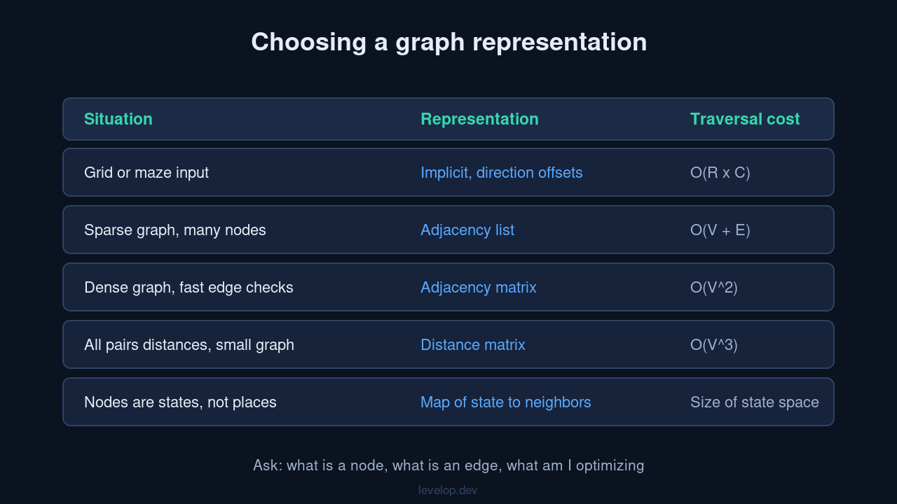
The last row deserves a moment, because it is the one that unlocks the hardest questions: nodes do not have to be places at all. In a word ladder the nodes are words and the edges are single letter changes, in a lock puzzle the nodes are dial configurations, and in a jug pouring puzzle the nodes are volume pairs. The moment you can express a problem as states plus legal transitions, breadth first search finds the fewest moves solution and the grid was never really the point.

Three questions to ask before you write code

Say these out loud in an interview, because they cost fifteen seconds and they reframe the entire problem.

1. What is a node? A cell, a word, a configuration, or a city index. Answering this fixes the shape of your visited set.
2. What is an edge? A direction offset, a one character edit, or a nonzero matrix entry. Answering this gives you the neighbor function.
3. What am I optimizing? Fewest steps points to breadth first search, connectivity or region shape points to depth first search, weighted cost points to Dijkstra, and every pair points to Floyd-Warshall.

Interviewers are grading the translation rather than the typing. A candidate who says this is connected components on an implicit grid graph, therefore depth first search with a visited set, linear in the number of cells, has already passed the part that matters, and the code that follows is mechanical.

Mistakes that cost real interviews

• Rebuilding an explicit adjacency list from a grid. It works, and it wastes both memory and the interviewer's patience. Compute neighbors on the fly.
• Forgetting that the visited set is the base case. Grid graphs contain cycles by construction, since any two by two block of open cells forms a loop, so a traversal without a visited set never terminates.
• Recursing on large grids. Convert depth first search to an explicit stack when the input can be large, or raise the recursion limit deliberately and say why.
• Reaching for Dijkstra on an unweighted graph. It returns the right answer while advertising that you did not notice the uniform cost.
• Mutating the input without mentioning it. Marking visited cells in place is a legitimate space optimization, but state that you are doing it and offer to restore the grid afterward.

If you want structured practice on these translations rather than random problem grinding, that is exactly what we built Levelop around, and there is more pattern breakdown on the Levelop blog.

References

Cormen, Leiserson, Rivest and Stein, Introduction to Algorithms, chapters on elementary graph algorithms and all pairs shortest paths. See also graph traversal on Wikipedia, adjacency matrix on Wikipedia, and 0-1 BFS on cp-algorithms.