

Advanced BFS: Multi-Source, Stateful, and Bidirectional
Back with another one in the pattern series. Plain BFS clicked for me a while ago: push the start node, pop, visit neighbors, repeat, done. Then I hit a wave of problems where that template just fell apart. A grid where rotten oranges spread from many cells at once. A maze where the shortest path depended on how many keys I was carrying. A word ladder that timed out until I searched from both ends. Same traversal, three completely different shapes.
That gap between "I know BFS" and "I can bend BFS to the problem" is what this post is about. Multi source BFS, stateful BFS, and bidirectional BFS are the three variations that show up over and over once the interview moves past the warm-up question.
Where basic BFS runs out
Basic BFS answers one question really well: what is the shortest number of edges from a single start node to everything else in an unweighted graph. You seed the queue with one node, you track visited, you expand level by level. If that is the whole problem, you are done.
The trouble starts when the problem breaks one of the hidden assumptions. What if there is no single start, but dozens of starting points firing at the same time? What if a cell is not simply visited or unvisited, but visited-while-holding-key-A versus visited-empty-handed? What if the graph is so wide that exploring from one side alone explodes into millions of nodes before you ever reach the target?
Each of those is a different assumption breaking. And each has a clean fix that is still just BFS underneath. That is the part I love. You are not learning three new algorithms. You are learning where to bend one.
Multi source BFS: start everywhere at once
The first variation is the one I reach for most. Multi source BFS is what you use when the shortest distance you care about is the distance to the nearest of several sources, not to one fixed origin.
The classic framing is the rotting oranges problem. You have a grid of fresh and rotten oranges. Every minute, a rotten orange rots its four fresh neighbors. You want the minute at which the last fresh orange rots. A naive approach runs a separate BFS from each rotten orange and takes the minimum distance per cell. That works, but it is wasteful and slow when there are many sources.
The insight that took me an embarrassingly long time to accept: you can put every source in the queue before the first pop. BFS does not care whether the queue starts with one node or five hundred. As long as every source enters at distance zero, the level-by-level expansion naturally computes the distance to the closest source for every cell at once.
from collections import deque

def oranges_rotting(grid):
    rows, cols = len(grid), len(grid[0])
    queue = deque()
    fresh = 0

    # Seed the queue with ALL rotten oranges at once
    for r in range(rows):
        for c in range(cols):
            if grid[r][c] == 2:
                queue.append((r, c))
            elif grid[r][c] == 1:
                fresh += 1

    minutes = 0
    while queue and fresh:
        minutes += 1
        for _ in range(len(queue)):   # process one full level
            r, c = queue.popleft()
            for dr, dc in ((1,0),(-1,0),(0,1),(0,-1)):
                nr, nc = r + dr, c + dc
                if 0 <= nr < rows and 0 <= nc < cols and grid[nr][nc] == 1:
                    grid[nr][nc] = 2
                    fresh -= 1
                    queue.append((nr, nc))

    return minutes if fresh == 0 else -1
The whole trick lives in that first loop. Seed everything, then run one ordinary BFS. The level-processing loop is what keeps the levels clean, so minutes increments exactly once per wave.
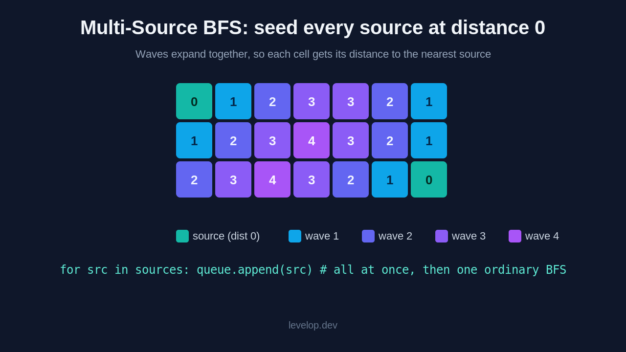
Once you see it, you start noticing multi source problems everywhere. Distance of every cell to the nearest zero in a matrix. Walls and gates where you fill each room with the distance to its closest gate. The shortest bridge problem, where you flood one island first, then run multi source BFS outward to reach the second. The tell is always the same: you want distance to the nearest of many things, not to one specific thing.
Stateful BFS: when a node is more than a coordinate
The second variation broke my mental model harder than the first. In basic BFS, "visited" is a boolean per node. You arrive at a cell, you mark it, you never come back. That works because arriving at a node is always equally good no matter how you got there.
Stateful BFS is for problems where that is false. Sometimes arriving at a cell carrying three keys is genuinely different from arriving at the same cell empty-handed, and you might need to visit that cell again in a better state. The node in your graph is no longer just a position. It is a position plus everything about your situation that affects the future.
The problem that forced me to internalize this is "shortest path to get all keys." You move through a grid, collect keys, and pass through locks only if you already hold the matching key. If you track visited as just (row, col), you will wrongly block yourself: you visit a cell early without a key, mark it seen, and then refuse to walk back through it later even though now you hold the key that opens the door beyond it.
The fix is to expand what "visited" means. The state becomes (row, col, keys_bitmask). Two visits to the same cell with different keys are different states, and both are allowed.
from collections import deque

def shortest_path_all_keys(grid):
    rows, cols = len(grid), len(grid[0])
    all_keys = 0
    start = None

    for r in range(rows):
        for c in range(cols):
            ch = grid[r][c]
            if ch == '@':
                start = (r, c)
            elif ch.islower():
                all_keys |= (1 << (ord(ch) - ord('a')))

    # State = (row, col, keys). Visited tracks states, not cells.
    seen = {(start[0], start[1], 0)}
    queue = deque([(start[0], start[1], 0, 0)])   # r, c, keys, steps

    while queue:
        r, c, keys, steps = queue.popleft()
        if keys == all_keys:
            return steps
        for dr, dc in ((1,0),(-1,0),(0,1),(0,-1)):
            nr, nc = r + dr, c + dc
            if not (0 <= nr < rows and 0 <= nc < cols):
                continue
            ch = grid[nr][nc]
            if ch == '#':
                continue
            if ch.isupper() and not (keys & (1 << (ord(ch.lower()) - ord('a')))):
                continue   # a lock we cannot open yet
            new_keys = keys
            if ch.islower():
                new_keys |= (1 << (ord(ch) - ord('a')))
            state = (nr, nc, new_keys)
            if state not in seen:
                seen.add(state)
                queue.append((nr, nc, new_keys, steps + 1))

    return -1
The bitmask is just a compact way to store which keys you hold. Key a is bit 0, key b is bit 1, and so on. A bitwise AND checks whether a bit is set, and a bitwise OR sets it. What matters more than the bit tricks is the mental shift: the moment you realize your visited set has to include the state, not just the position, the whole family of problems opens up.
Stateful BFS shows up whenever the cost of the future depends on more than where you are standing. Grids with a limited number of allowed obstacle eliminations. Puzzles where you track direction and turn count. Anything where you would naturally say "it depends what I'm carrying." The extra dimensions in the state are exactly the things that change what you can do next.
Bidirectional BFS: meet in the middle
The third variation is a pure performance play. Bidirectional BFS does not solve a problem that plain BFS cannot. It solves the same problem far faster when the graph fans out widely.
Think about the shape of a BFS frontier. From a single start, the number of nodes at distance d grows roughly like the branching factor b raised to the power d. If the answer is at depth d, you touch on the order of b to the d nodes. That exponent is what kills you on wide graphs like word ladders, where every word has many one-letter neighbors.
Bidirectional BFS attacks the exponent directly. Instead of one search of depth d, you run two searches of depth d over 2, one forward from the start and one backward from the target, and you stop the moment their frontiers touch. Two searches of b to the d over 2 are dramatically smaller than one of b to the d. Halving the exponent is the whole game.
The mechanics matter here, because it is easy to write a version that looks right and gives wrong answers. You keep two frontiers as sets. On each round you always expand the smaller frontier, which keeps both sides balanced. After expanding, you check whether any newly reached node already lives in the other side's visited set. If it does, the two searches have met and the total distance is the sum of the two half-distances.
def ladder_length(begin, end, word_list):
    words = set(word_list)
    if end not in words:
        return 0

    front, back = {begin}, {end}
    seen = {begin, end}
    steps = 1

    while front and back:
        # Always expand the smaller frontier
        if len(front) > len(back):
            front, back = back, front

        nxt = set()
        for word in front:
            for i in range(len(word)):
                for ch in 'abcdefghijklmnopqrstuvwxyz':
                    cand = word[:i] + ch + word[i+1:]
                    if cand in back:
                        return steps + 1     # frontiers met
                    if cand in words and cand not in seen:
                        seen.add(cand)
                        nxt.add(cand)
        front = nxt
        steps += 1

    return 0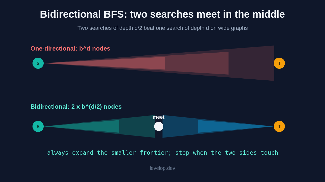
The swap that always expands the smaller set is not a nice-to-have. It is what keeps the two sides growing at the same rate and preserves the performance win. Skip it and one frontier can balloon while the other starves, and you are back to something close to a single-directional search.
Bidirectional BFS has real preconditions, though. You need to know the target node up front, since you have to search backward from it. You need to be able to generate predecessors, which is trivial in undirected graphs and grids but awkward in directed ones. And the payoff only shows up when the branching factor is high enough that the exponent actually hurts. For a narrow graph, the bookkeeping is not worth it.
How to tell which variation a problem wants
After enough reps, a quick decision process emerged for me, and it takes only a few seconds at the start of a problem.
If the shortest distance is measured to the nearest of several origins, that is multi source BFS. Seed the queue with all of them at distance zero. If arriving at a node in different circumstances leads to different futures, that is stateful BFS. Push the circumstances into the state and let your visited set track states. If you have one start, one known target, a wide branching factor, and plain BFS is too slow, that is bidirectional BFS. Search from both ends and meet in the middle.
They also stack. It is completely normal to run a multi source search where each node also carries state, or to reason about a stateful search using the same level-counting skeleton. Underneath, all three are the same loop: a queue, a visited set, and level-by-level expansion. The variations only change what goes into the queue and what counts as already seen.
That framing is what finally made these feel like one pattern with three settings instead of three things to memorize. It is the same idea behind why Levelop teaches twelve patterns instead of grinding twenty-five hundred problems: once you see the shared skeleton, the variations stop being separate homework.
What to practice next
A short, ordered path that mirrors how the difficulty ramps:
Start with rotting oranges and 01 matrix to lock in multi source seeding. Both are pure "distance to nearest source" problems and cheap to reason about. Then move to walls and gates and shortest bridge, which combine multi source BFS with a bit of setup work before the search.
For stateful BFS, do shortest path in a grid with obstacle elimination first, since the state is just one extra integer. Then take on shortest path to get all keys, where the bitmask state makes the pattern unavoidable.
For bidirectional BFS, word ladder is the canonical exercise. Write the single-directional version first, watch it strain on large inputs, then rewrite it from both ends and feel the difference. If you want the broader map of how these relate to depth-first and dynamic programming approaches, the BFS vs DFS vs DP comparison is a good next read, and the DFS with memoization walkthrough shows what changes when caching enters the picture.
Frequently Asked Questions
What is the difference between BFS and multi source BFS?
There is no difference in the algorithm itself. Multi source BFS is ordinary BFS where you push every source node into the queue before the first pop, all at distance zero. The level-by-level expansion then computes the shortest distance from each node to its nearest source in one pass, instead of running a separate BFS from each source.
When should I use bidirectional BFS instead of regular BFS?
Use bidirectional BFS when you have a single known start and a single known target, the graph has a high branching factor, and a normal BFS explores too many nodes. Searching from both ends turns roughly b to the d work into two searches of b to the d over 2, which is a large saving on wide graphs like word ladders. It needs a known target and the ability to generate predecessors, so it does not fit every problem.
What does state mean in stateful BFS?
State is everything about your current situation that changes what you can do next, beyond your position. In a keys-and-locks grid, the state is your coordinates plus which keys you hold. Your visited set tracks states rather than bare positions, which lets you revisit a cell when you arrive in a genuinely better situation.
Why does my BFS give wrong answers on grids with keys or obstacles?
Almost always because you are marking cells visited by coordinate alone. When the future depends on more than position, two visits to the same cell in different states are different, and blocking the second one cuts off the only valid path. Include the state in your visited set and the bug disappears.
Can I combine these BFS variations in one problem?
Yes, and harder problems often expect it. You can run a multi source search where each queued item also carries state, or apply level counting inside a bidirectional search. They all share the same queue-and-visited skeleton, so the variations compose cleanly. What changes is only what you put in the queue and what you treat as already seen.
Wrapping up
The jump from textbook BFS to interview BFS is not about learning new algorithms. It is about recognizing which assumption a problem breaks and bending the same traversal to fit. Multi source when distance is to the nearest of many. Stateful when the situation, not just the position, drives the future. Bidirectional when the graph is too wide to search from one side. One loop, three settings.
If you want a structured way to drill these instead of hunting for problems one at a time, this breakdown came out of the graph traversal track on Levelop, where the advanced BFS problems are grouped by exactly these variations. More pattern breakdowns are on the Levelop blog.
References
- LeetCode, Rotting Oranges and Shortest Path to Get All Keys problem sets, leetcode.com.
- CP-Algorithms, Breadth-first search and 0-1 BFS, cp-algorithms.com.
- Cormen, Leiserson, Rivest and Stein, Introduction to Algorithms, breadth-first search chapter.
- Levelop, BFS vs DFS vs DP and the graph traversal pattern track, levelop.dev/blog.