BFS vs DFS vs DP: When to Use Which to Explore a Search Space

Most interview prep treats breadth first search, depth first search, and dynamic programming as three unrelated topics. You grind BFS problems one week, DFS problems the next, then hit a wall of DP problems that feel like a different universe. That framing is why so many candidates freeze on a problem they could actually solve. The truth is simpler and more useful: these are three ways to explore a search space. Once you see them that way, deciding BFS vs DFS vs DP when to use each one becomes a short, repeatable decision instead of a guess.

This post gives you that decision. We will define the search space idea, walk through what each technique is really optimizing for, and give you a concrete checklist you can run in the first two minutes of any problem.

The one idea that connects all three: a search space

Almost every algorithmic problem can be phrased as a space of possible states that you need to move through to find something. A state might be a cell in a grid, a node in the graph, a substring, a subset, or a partial solution you are building up. The edges in the graph between states are the legal moves: step to a neighbor cell, follow a graph edge, add one more character, or include or exclude one more item.

Under this lens, the three techniques differ only in how they walk the space and what they remember. Two of them are graph traversal algorithms, and the third is a memory strategy that sits on top of a traversal.

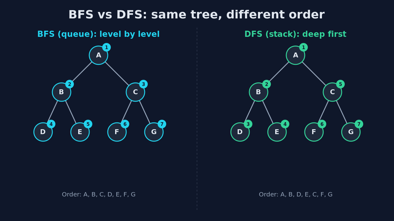
Breadth first search explores the space in rings, level by level, closest states first. Depth first search plunges down one path as far as it can, then backtracks. Dynamic programming does not really care about traversal order at all. It cares about not recomputing the same state twice. Getting BFS vs DFS right is a question of traversal order. Getting DP right is a question of overlap and reuse.

BFS: when the shortest path or nearest layer matters

Breadth first search bfs visits states in order of distance from the start node. It uses a queue data structure, so the first time it reaches a state, it has reached it by the fewest number of moves. That single property is the whole reason BFS exists, and it is why BFS traversals are the default tool for distance questions.

Reach for BFS when the question contains any of these signals: shortest path in an unweighted graph, minimum number of steps, fewest moves, nearest target, or level by level processing of a tree.

from collections import deque

def shortest_path(grid, start, target):
    rows, cols = len(grid), len(grid[0])
    queue = deque([(start, 0)])
    seen = {start}                       # track every visited node
    while queue:
        (r, c), dist = queue.popleft()
        if (r, c) == target:
            return dist
        for dr, dc in ((1, 0), (-1, 0), (0, 1), (0, -1)):
            nr, nc = r + dr, c + dc
            if 0 <= nr < rows and 0 <= nc < cols and grid[nr][nc] == 0 and (nr, nc) not in seen:
                seen.add((nr, nc))
                queue.append(((nr, nc), dist + 1))
    return -1

The moment you dequeue the target, the distance is guaranteed minimal because every state at distance k is dequeued before any state at distance k plus 1. The seen set marks each node visited so you never enqueue it twice, which keeps the time complexity at O(V + E) for a graph stored as adjacency lists.

BFS also shines for flood fill style problems: counting islands, spreading infection or rot across a grid one minute at a time, or finding the nearest exit. Anything where a wave expanding outward matches the problem is a BFS problem.

DFS: when you need to exhaust paths, backtrack, or explore structure

Depth first search dfs commits to one path and follows it until it dead-ends, then unwinds. It uses recursion or an explicit stack. DFS does not find shortest paths in general, and trying to force it to is a classic mistake. When you traverse the graph this way, you go deep before you go wide.

Reach for DFS when the question involves exploring all paths or configurations, detecting cycles, topological ordering, connected components where distance does not matter, or building and unwinding partial solutions through backtracking.

def all_paths(graph, start, target):
    results = []
    def walk(node, path):
        if node == target:
            results.append(path[:])
            return
        for nxt in graph[node]:          # graph is an adjacency list
            path.append(nxt)
            walk(nxt, path)
            path.pop()                   # backtrack: undo the choice
    walk(start, [start])
    return results

That path.pop() call is the heart of backtracking. You make a choice, recurse, then undo the choice so the next branch starts clean. Permutations, combinations, subsets, N-Queens, Sudoku, and word-search problems are all DFS with backtracking. If the problem asks for every valid arrangement rather than the best single number, you are almost always in DFS territory.

DFS algorithms are also the natural fit when you care about structure rather than distance. Counting connected components in an undirected graph, checking whether a graph is bipartite, or producing a topological sort all lean on the depth first traversal order and the recursion stack. A DFS traversal touches the same data structures as BFS, just in a different order.

The overlap: many problems accept either BFS or DFS

For "is this reachable" or "how many connected components" questions, distance is irrelevant, so BFS vs DFS when to use comes down to convenience and constraints. When to use BFS vs DFS in that case is a coin flip weighted by your input size.

DFS is often shorter to write recursively. BFS avoids deep recursion and the stack overflow risk that comes with it on large inputs. If the graph could be tens of thousands of nodes deep, prefer the iterative BFS or an explicit stack so you do not blow the call stack. Both approaches show how the same graph traversal algorithms adapt to different limits.

DP: when the search space has massive overlap

Dynamic programming is a different axis entirely. BFS and DFS answer how you walk the space. DP answers how you avoid walking the same corner of the space a thousand times.

You reach for DP when a brute-force recursion would revisit the same state over and over. The technical name for the two conditions is overlapping subproblems and optimal substructure. In plainer terms, the same smaller question keeps coming up, and the best answer to the big question is built from the best answers to those smaller questions.

The canonical example is Fibonacci. Naive recursion recomputes fib(3) an exponential number of times. Caching each result the first time and reusing it collapses the work to linear time complexity.

from functools import lru_cache

@lru_cache(maxsize=None)
def fib(n):
    if n < 2:
        return n
    return fib(n - 1) + fib(n - 2)

Notice what DP does not specify: the traversal order. Top-down cached DP is literally a DFS through the state space with a cache bolted on. Bottom-up tabulated DP fills states in dependency order, which often looks like a BFS or a simple loop. This is why DP feels slippery at first. It is not a competing traversal, it is a memory strategy layered on top of one.

We go deeper on this in dynamic programming is state plus transition, not memorization, which reframes DP around defining the state cleanly. The related piece on turning recursion into dynamic programming with memoization shows the mechanical step from a plain DFS to a cached one.

BFS vs DFS vs DP when to use: the two-minute decision checklist

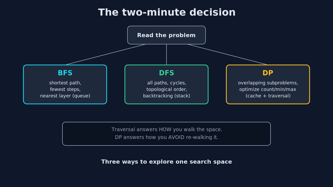
Here is the exact sequence to run when you first read a problem. It takes under two minutes and resolves most cases.

First, ask what the problem wants. If it wants the shortest path, minimum steps, or nearest layer in an unweighted graph, use BFS and stop. That property is unique to BFS and worth reaching for immediately.

Second, if it wants all configurations, cycle detection, topological order, or connected structure where distance is irrelevant, use DFS, usually with backtracking if you are building solutions.

Third, ask whether a brute-force recursion would recompute the same state. If yes, and you are optimizing a count, a max, a min, or a number of ways, add caching and you are doing DP. The presence of "how many ways," "minimum cost," or "maximum value" over choices is a strong DP tell.

Fourth, watch for combinations. Many hard problems are DP layered over a DFS, or a BFS where each state is itself computed with DP. The techniques compose. Recognizing the base traversal first, then asking whether overlap exists, keeps you from conflating them.

Quick reference

BFS is for shortest path and level by level order on unweighted graphs, backed by a queue data structure, with the key property that the first visit is the closest visit. DFS is for exhaustive exploration, backtracking, cycles, and topological sort, backed by a stack or recursion, with no shortest-path guarantee. DP is for overlapping subproblems and optimization, backed by a cache or table, and it rides on top of either traversal rather than replacing it. All three read the same node in the graph and the same edges in the graph, so the underlying data structures rarely change. Only the order and the memory do.

A worked example that touches all three

Consider a classic: given a grid, count the number of distinct shortest paths from the top-left to the bottom-right, moving only right or down, avoiding blocked cells.

The word "shortest" hints at BFS, but because movement is only right or down, every path from start to end has the same length, so shortest is automatic. The word "count the number of distinct paths" is the real signal. That is a "how many ways" phrasing, which points to DP.

def count_paths(grid):
    rows, cols = len(grid), len(grid[0])
    dp = [[0] * cols for _ in range(rows)]
    dp[0][0] = 1 if grid[0][0] == 0 else 0
    for r in range(rows):
        for c in range(cols):
            if grid[r][c] == 1:      # blocked cell
                dp[r][c] = 0
                continue
            if r > 0:
                dp[r][c] += dp[r - 1][c]
            if c > 0:
                dp[r][c] += dp[r][c - 1]
    return dp[rows - 1][cols - 1]

A pure DFS here would explore an exponential number of paths and time out. The DP version fills each cell once, reusing the counts of the cells above and to the left. Same search space, but the overlap made DP the correct exploration strategy. This is exactly the reasoning our DP archetypes guide trains you to run automatically.

Why this framing beats memorizing problem lists

The reason we teach patterns rather than problem counts at Levelop is that a candidate who has memorized two hundred BFS problems still stalls when a problem does not look like any of them. A candidate who understands that these are three ways to explore a search space can classify a brand-new problem in the first two minutes. That is the difference between pattern recognition and rote recall, and it is the whole argument behind teaching 12 patterns instead of 2500 problems.

For the underlying theory, the treatment of graph traversal algorithms and dynamic programming in the standard reference, Introduction to Algorithms by Cormen, Leiserson, Rivest, and Stein, is worth reading once slowly. The traversal chapters make the queue-versus-stack distinction rigorous. The DP chapter formalizes overlapping subproblems in a way that sticks.

Common mistakes to avoid

The first mistake is using DFS for a shortest-path problem and hoping it works. It will return a path, just not the shortest one, and you will lose points.

The second is forcing BFS onto a problem that needs all configurations. The queue explodes because you are trying to enumerate exponentially many states level by level.

The third, and most common in DP, is failing to define the state precisely before writing code. If you cannot state what one cell of your table means in a single sentence, you are not ready to write the recurrence.

Browse the full Levelop blog for pattern-by-pattern breakdowns that drill each of these into muscle memory.