
Latency vs Throughput: Numbers Engineers Must Know
Two engineers look at the same dashboard. One says the system is slow. The other says it is fast. Both are right. One is watching latency. The other is watching throughput. Confusing the two is one of the most common mistakes in system design interviews and production postmortems.
Latency and throughput sit underneath almost every architectural decision. Should you add a cache? Batch your writes? Shard the database? Each choice moves latency or throughput, often at the expense of the other. Without an intuition for the numbers, you are guessing. This post fixes that. We define latency vs throughput, list the latency numbers every programmer should know, place bandwidth in context, and use the numbers for real estimates.
Latency vs Throughput, Defined
Latency is the time a single operation takes, from request to response. You measure it in time: nanoseconds, microseconds, milliseconds. Lower is better.
Throughput is the number of operations completed per unit of time. You measure it in operations per second: queries per second (QPS), requests per second, megabytes per second. Higher is better.
Picture a highway. Latency is how long one car takes to cross it. Throughput is how many cars pass a point each minute. More lanes raise throughput without changing any single trip. A higher speed limit lowers latency for every car. They are related, but they are different dials.
Here is the catch. Improving one often hurts the other. Batching a hundred writes into one transaction raises throughput by amortizing fixed costs. It also raises latency for the first write, which now waits for ninety-nine others. That tension is the heart of performance work.
The Latency Numbers Every Programmer Should Know
In 2009, Jeff Dean of Google popularized a table of numbers everyone should know, and Peter Norvig published a similar set. Exact values shift with hardware, but the orders of magnitude stay stable. Memorize the shape, not the last digit.
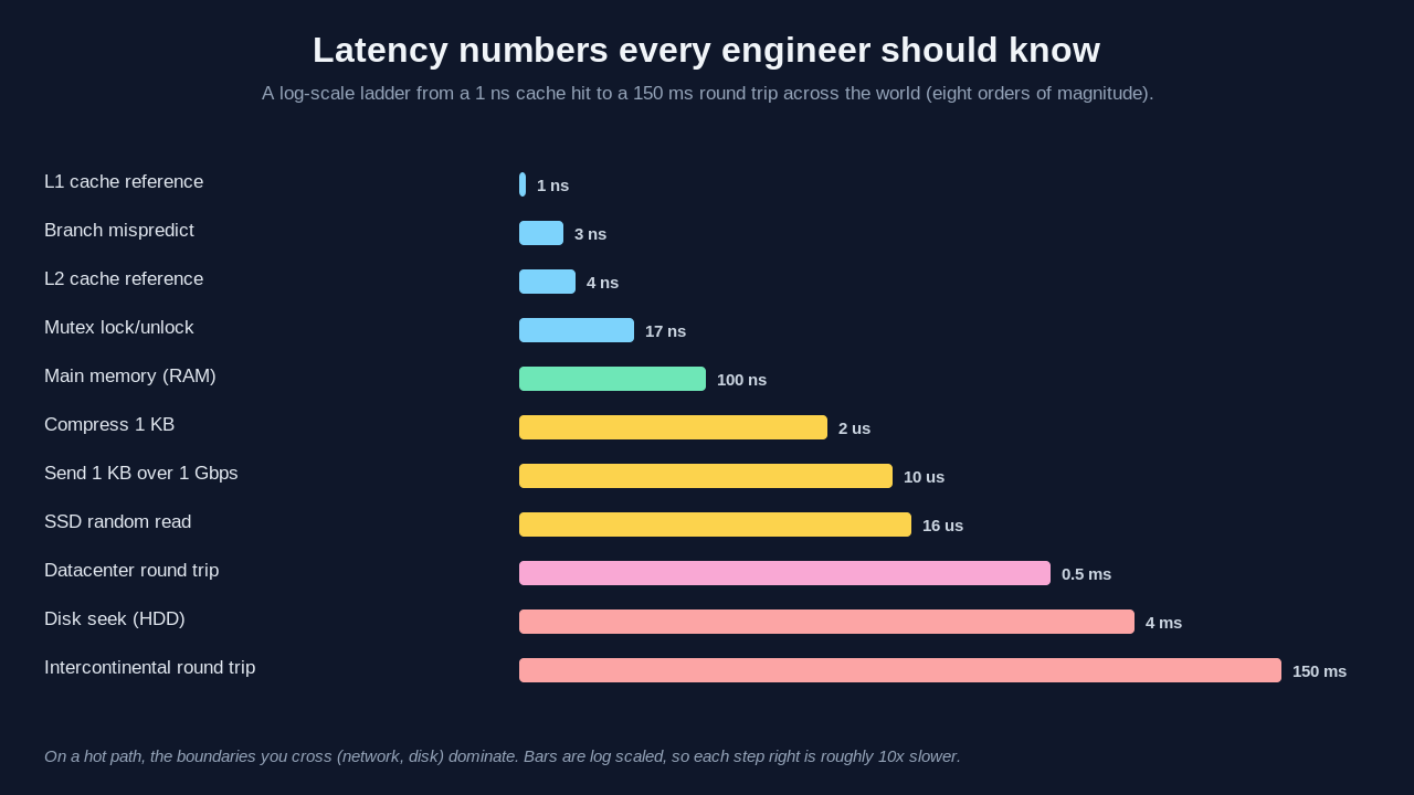
Operation                     Latency          x L1
L1 cache reference            1 ns             1x
Branch mispredict             3 ns             3x
L2 cache reference            4 ns             4x
Mutex lock/unlock             17 ns            17x
Main memory (RAM)             100 ns           100x
Compress 1 KB, fast codec     2,000 ns         2,000x
Send 1 KB over 1 Gbps         10,000 ns        10,000x
SSD random read               16,000 ns        16,000x
Datacenter round trip         500,000 ns       500,000x
Disk seek (HDD)               4,000,000 ns     4,000,000x
Intercontinental round trip   150,000,000 ns   150,000,000x
Notice the jumps. RAM is about a hundred times slower than L1. An SSD read is over a hundred times slower than RAM. A datacenter round trip is thirty times slower than that SSD read. Crossing an ocean is another three hundred times slower. The table spans eight orders of magnitude.
A human-scale analogy helps. Say one L1 reference took one second. Then RAM would take a minute and a half. An SSD read would take four and a half hours. A datacenter round trip would take almost a week. The intercontinental round trip would take nearly five years. Brendan Gregg uses this scaling in his book Systems Performance to show why one cache miss in a hot loop can dominate everything.
Where Bandwidth Fits In
People say "fast network" and mean two different things. That is why throughput vs bandwidth vs latency is worth pinning down.
Bandwidth is the maximum rate a link can carry, a property of the pipe: a 1 Gbps link, a 100 Gbps backbone. Throughput is the rate you actually achieve, always less than bandwidth because of overhead, congestion, and round trips. Latency is the delay before the first byte arrives.
The pipe analogy is clean. Bandwidth is the pipe diameter. Latency is the pipe length. Throughput is how much water flows per second once it runs. A wide, long pipe has high bandwidth and high latency at once. Picture a truck of hard drives crossing the country: huge bandwidth, a full day of latency. This is why high throughput vs low latency is not a contradiction. A batch analytics job wants throughput and tolerates latency. An online game wants low latency and needs only modest throughput.
The Latency vs Throughput Tradeoff
Three techniques appear again and again, and each trades these numbers against each other. Batching groups small operations into one larger operation. It raises throughput by amortizing fixed costs like round trips and disk seeks. It raises tail latency because operations wait to be grouped. Kafka producers and bulk inserts batch for this reason.
Pipelining overlaps stages of independent operations so the system is never idle. A CPU pipeline does not make one instruction finish faster, so latency per instruction is unchanged. It raises instruction throughput sharply. Queueing absorbs bursts so a downstream service sees smooth load. A queue protects throughput under spikes, but every item waits in line, which adds latency. Little's Law governs this.
Little's Law:   L = lambda x W

L      = average items in the system (concurrency)
lambda = average arrival rate (throughput)
W      = average time in the system (latency)
For a fixed concurrency, throughput and latency are inversely linked. To push more requests per second through a server that holds only so many in flight, the time each request spends inside must drop, or the queue and its latency must grow. There is no free lunch.
Estimate: Storage for 1 Million Users
Now put the numbers to work. You are designing a social app and want a storage estimate for one million users. The goal is not precision. It is being right within an order of magnitude, fast.
Start per user. Say a user record holds a profile and metadata, roughly 2 KB. For a million users that is 2 GB. That fits in one server's RAM. Now add content. Say each user posts 100 items at 1 KB each. That is 100 KB per user, or 100 GB total. Still one beefy database node.
Images explode the estimate. If each user uploads 50 images at 500 KB, that is 25 MB per user, or 25 TB total. Text was a rounding error next to media. That is the key lesson of capacity estimation: find the dominant term and design for it. You store text in Postgres and images in object storage behind a CDN, because the numbers say so. For worked examples covering DAU, QPS, cache, and bandwidth, see our deep dive on back-of-the-envelope estimation.
Estimate: QPS of a Single Server
The second favorite interview question: how many queries per second can one server handle? The honest answer is that it depends on the query. You show skill by reasoning from the latency table.
A request served from memory might do 100 microseconds of work. One core could in theory handle 10,000 requests per second. An eight-core box might sustain tens of thousands of QPS for cache-served traffic. Now add an SSD read at 16 microseconds. With a few reads plus compute, real work climbs to a few hundred microseconds, dropping you toward 2,000 to 5,000 QPS per core.
Now cross the network: 500 microseconds per datacenter round trip. Two serial calls cost 1 millisecond of pure waiting, capping you near 1,000 requests per second per worker before compute. That is why cutting sequential network hops, through caching, batching, or parallel fan-out, is so often the highest-leverage optimization. Throughput per server falls with the slowest operation each request performs.
How This Shows Up in Interviews
When an interviewer asks you to design a system, latency vs throughput system design reasoning separates a senior answer from a junior one. A junior candidate jumps to technologies. A senior candidate first asks which number matters: a read-heavy, latency-sensitive feed that needs caching, or a write-heavy, throughput-sensitive pipeline that needs queues.
State your targets out loud. Estimate the load. Identify the dominant cost with the latency table. Then choose components. That order is what interviewers at Amazon, Google, and Meta score. For the full playbook, see the Levelop blog.
Conclusion
Latency is how long one operation takes. Throughput is how many you finish per second. Bandwidth is the ceiling on the pipe, not the speed you see. The latency numbers span eight orders of magnitude, and the boundaries you cross in a hot path are where the time goes. Internalize the table, reason from the dominant term, and state which number you optimize. Explore more fundamentals on Levelop.
Frequently Asked Questions
What is the difference between latency and throughput?
Latency is the time a single operation takes, from request to response, measured in time units. Throughput is how many operations finish per second. Latency describes one trip; throughput describes the flow of many. You can improve one without the other, and batching often raises throughput while raising latency.
Are latency and throughput inversely related?
Not always, but they are linked through concurrency by Little's Law. For a fixed number of in-flight operations, more throughput forces either lower per-operation latency or a longer queue. Adding parallel capacity can raise throughput without hurting latency, so it depends on your bottleneck.
What are the latency numbers every programmer should know?
Roughly: L1 cache 1 ns, main memory 100 ns, SSD random read 16 us, a datacenter round trip 0.5 ms, a disk seek 4 ms, and an intercontinental round trip 150 ms. Exact values change with hardware, but the orders of magnitude and the gaps between tiers stay stable.
Is bandwidth the same as throughput?
No. Bandwidth is the maximum rate a link can carry, a fixed property of the connection. Throughput is the rate you actually achieve, always lower because of overhead, congestion, and round-trip delays. Bandwidth is the pipe width; throughput is how much water flows through per second.
How do I estimate the QPS a single server can handle?
Estimate the work per request from the latency table, then divide one second by it. An in-memory request near 100 us implies about 10,000 QPS per core. An SSD read drops it to a few thousand. A couple of serial network round trips drop it toward 1,000 per worker. The slowest operation sets the ceiling.
References
- Jeff Dean, "Numbers Everyone Should Know," Google design lectures, 2009.
- Peter Norvig, "Teach Yourself Programming in Ten Years," norvig.com.
- Brendan Gregg, "Systems Performance: Enterprise and the Cloud," 2nd edition.
- Martin Kleppmann, "Designing Data-Intensive Applications," O'Reilly.
- John D. C. Little, "A Proof for the Queuing Formula," Operations Research, 1961.