Uber System Design: Geospatial Matching, Surge Pricing, ETA

"Design Uber" is one of those interview prompts that sounds simple until you start drawing boxes. A rider taps a button, a nearby driver appears, a price shows up, and a little car slides across a map toward a pin. Four smooth seconds of product hide a genuinely hard distributed system underneath. The first time I tried to whiteboard the uber system design question, I got about two minutes in before I realized I had no idea how the app finds nearby drivers without scanning every driver on the planet.

This post walks through the real system behind the ride, the same way I eventually learned to reason about it. We will frame the problem, run a back-of-the-envelope estimate, then dig into the three parts that make a system design of uber application interesting: geospatial matching, surge pricing, and ETA prediction. By the end you should be able to design uber system design confidently at a whiteboard, and more importantly understand why each piece exists.

What "design Uber" actually asks

Before drawing anything, separate what the system must do from how well it must do it. When an interviewer says "design uber," they are really asking you to reason about matching supply to demand in physical space, in real time, at scale.

The functional requirements are the visible product. A rider requests a ride from a pickup location. The system finds nearby available drivers and matches one to the request. Both parties see each other move on a live map. The rider sees a fare estimate before confirming and a final price after. The system predicts an arrival time for both the pickup and the destination.

The non-functional requirements are where the design earns its difficulty. Matching has to feel instant, so the nearby-driver lookup needs to return in well under a second. The service has to stay available across cities and time zones, because an outage means stranded riders and idle drivers losing income. Location data arrives continuously from millions of moving cars, so the write path has to absorb a firehose of updates. And the whole thing is geographically partitioned by nature: a rider in Berlin never needs to be matched with a driver in Bogota.

Back-of-the-envelope: sizing the firehose

A quick estimate tells you which parts of the design are hard. Suppose the platform has around 5 million active drivers online at peak. Each driver's phone reports its location every 4 seconds while they are available.

active_drivers = 5_000_000
seconds_between_updates = 4

location_writes_per_second = active_drivers / seconds_between_updates
print(location_writes_per_second)  # 1,250,000 writes/sec

That is over a million location writes per second, sustained. If you tried to push each one into a traditional relational row and index it on latitude and longitude, the index maintenance alone would fall over. This single number is why ride-hailing systems keep live location in memory, in a structure built for spatial queries, rather than in a general-purpose database. On the read side, ride requests are far rarer than location updates, three orders of magnitude smaller than the write load. That asymmetry, heavy writes and comparatively light reads, shapes every decision that follows. If you want a refresher on turning assumptions into numbers like this, our walkthrough of back-of-the-envelope calculation covers the method in detail.

Ingesting location: why a SQL table will not do

Picture the naive approach. Every driver update runs an UPDATE on a drivers row by id, and matching runs a bounding-box SELECT filtering latitude between two values and longitude between two values. Two problems show up immediately.

First, the write volume we just estimated destroys a B-tree index that has to be re-balanced on every coordinate change. Second, a bounding-box query on latitude and longitude cannot use a single index efficiently, because the two columns are independent. The database ends up scanning a huge candidate set and filtering it in memory.

The fix is to treat the map itself as the index. Instead of storing raw coordinates and searching them, you convert every location into a key that encodes where it sits in space, so that "nearby in the world" becomes "nearby in the key space." That is the idea behind geospatial indexing, and it is the core trick of the whole design.

Geospatial matching: turning the map into an index

There are two dominant families of spatial index in production ride-hailing systems: geohashing and tree-based grids. They solve the same problem, so it helps to understand both.

Geohashing

A geohash encodes a latitude and longitude pair into a short string by repeatedly dividing the world into a grid and recording which cell the point falls into. The elegant property is that points close together in the world usually share a common string prefix. San Francisco's Mission District might sit in one cell, and two points a few blocks apart share that prefix while a point across the bay differs earlier in the string.

import pygeohash as pgh

# Encode a driver's position to a 6-char cell (about 1.2km x 0.6km)
driver_cell = pgh.encode(37.7599, -122.4148, precision=6)  # '9q8yyk'

# To find nearby drivers, look up the rider's cell plus its 8 neighbors,
# then fetch every driver keyed under those 9 cells from Redis.
def nearby_cells(rider_lat, rider_lng, precision=6):
    center = pgh.encode(rider_lat, rider_lng, precision=precision)
    return [center] + pgh.neighbors(center)

At request time, you compute the rider's geohash, gather that cell and its eight neighbors (so you do not miss a driver just across a cell boundary), and pull the drivers keyed under those cells. Because the drivers are held in an in-memory store like Redis keyed by geohash cell, this lookup is a handful of key reads rather than a table scan. If you have read our piece on consistent hashing and virtual nodes, the same partitioning instinct applies here: you shard the live location data by geographic cell so no single node holds the whole world.

Quadtrees and hierarchical grids

The precision of a geohash is fixed by its length, which is awkward. Downtown Manhattan and rural Montana get the same cell size even though one holds thousands of drivers and the other holds none. Quadtrees fix this by subdividing space adaptively: a cell splits into four children only when it holds more than some threshold of drivers. Dense areas get fine-grained cells, empty areas stay coarse.

Google's S2 library and Uber's own H3 hexagonal grid are production-grade versions of this idea. H3 tiles the world in hexagons because hexagons have uniform distance to all neighbors, which makes "expand my search ring outward" cleaner than it is with squares. The tradeoff is that a tree needs rebalancing as drivers move between cells, whereas a flat geohash scheme is simpler to update. Many real systems combine both: a flat cell key for the hot write path and a hierarchical grid for smarter search radius expansion.

The matching service: from nearby to chosen

Finding nearby drivers is only half of matching. Once you have a candidate set of, say, twenty available cars within a couple of kilometers, you have to pick one. Naive distance ranking is a decent start, but real dispatch considers driver rating, direction of travel, estimated pickup time given traffic, and whether assigning this driver strands demand elsewhere.

A common pattern is to keep matching stateful per geographic region. A dispatch worker owns a set of cells, holds the live driver index for those cells in memory, and processes ride requests for that region off a queue. This keeps the hot data local and lets you scale by adding workers per region rather than one giant global matcher. When a request comes in, the worker filters candidates, ranks them, sends an offer to the top driver, and falls back to the next if the offer times out.

Because offers and acceptances happen over the network with humans in the loop, the matching flow is naturally asynchronous. Understanding when to block and when to fire-and-forget matters here, and our explainer on synchronous versus asynchronous communication is a useful companion for reasoning about the request path.

Surge pricing: supply and demand in real time

Surge pricing is the system's way of nudging supply and demand back into balance. When too many riders chase too few drivers in an area, the price rises, which suppresses some demand and pulls in nearby drivers. It is an economic feedback loop implemented as a streaming computation.

Conceptually, each geographic cell tracks two rolling counts over a short window: open ride requests and available drivers. The surge multiplier is a function of the ratio between them.

def surge_multiplier(open_requests, available_drivers):
    if available_drivers == 0:
        return 3.0  # capped ceiling when supply is exhausted
    demand_ratio = open_requests / available_drivers
    if demand_ratio <= 1.0:
        return 1.0
    # Smoothly scale up, capped so prices never spike absurdly
    return min(1.0 + 0.5 * (demand_ratio - 1.0), 3.0)

The hard part is not the formula, it is computing it continuously per cell across a whole city without lag. This is a stream-processing job: location and request events flow into a system like Kafka, a processor maintains windowed counts per cell, and the resulting multipliers are written to a fast store that the pricing service reads at quote time. Multipliers are cached with short expiries because a stale surge value either overcharges riders or fails to attract drivers. Our overview of caching strategies for system design covers the expiry and invalidation tradeoffs that make or break this layer.

ETA prediction: from straight lines to machine learning

The arrival time estimate looks like a small feature and is secretly one of the deepest parts of the system. A straight-line distance divided by average speed is wildly wrong in a city with one-way streets, rivers, and rush hour. Real ETA prediction has three layers.

First, a routing engine computes the actual road-network path between two points, not the geometric distance. This is a shortest-path search over a graph of road segments, typically precomputed and heavily optimized because it runs constantly.

Second, each road segment carries a live speed estimate derived from the location traces of drivers currently on it. The system is its own traffic sensor: millions of moving cars continuously report how fast each street actually is right now.

Third, a machine-learning model corrects the routing estimate using historical patterns, weather, time of day, and event data. The model learns that a particular intersection is always slow at 6 p.m. on Fridays, something a pure graph search cannot know.

Putting the architecture together

Zoom out and the system design of uber application resolves into a handful of cooperating services. A location ingestion service absorbs the driver update firehose and maintains the in-memory geospatial index, sharded by region. A matching service reads that index to find and rank candidate drivers per request. A pricing service reads streaming supply-and-demand counts to compute fares. An ETA service combines routing, live traffic, and an ML model. A trip service tracks the ride lifecycle once a match is made and writes durable records for billing.

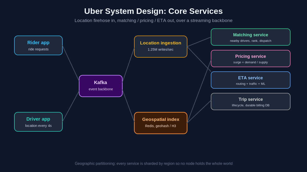
Between them sits a streaming backbone, usually Kafka, carrying location events, ride requests, and trip state changes. The live spatial and surge data lives in an in-memory store like Redis for speed, while durable trip and billing records land in a partitioned database. The same in-memory sorted-structure approach that powers a Redis leaderboard for millions of players shows up here for ranking nearby drivers by distance. And because every service depends on that stream of location events, the design leans heavily on asynchronous, event-driven communication rather than tight synchronous calls.

Common mistakes in the Uber system design interview

The first mistake is jumping straight to microservices and databases without addressing the geospatial index. That index is the whole problem; skip it and you have designed a generic CRUD app. The second is proposing a raw SQL query on latitude and longitude, which shows you have not internalized the write volume. The third is treating surge and ETA as trivial formulas rather than streaming and ML systems. The fourth is forgetting the geographic partitioning that makes the system scale in the first place. If you frame the problem around the spatial index and let matching, pricing, and ETA hang off it, you will design uber system design in a way that holds up to follow-up questions.

Wrapping up

The reason "design Uber" endures as an interview question is that it forces you to reason about physical space, real-time streams, and economic feedback all at once. Keep the spatial index at the center, size the write firehose early, and treat surge and ETA as the streaming and ML systems they really are. If you want to keep sharpening your system design instincts, browse more walkthroughs on the Levelop blog, or head back to Levelop to see how we help engineers prepare.

References

For deeper background on the spatial data structures behind this design, Uber's engineering write-up on the H3 hexagonal grid is worth a read.

1. Uber Engineering, H3: Uber's Hexagonal Hierarchical Spatial Index, uber.com/blog/h3.
2. Levelop, Back of the Envelope Calculation and Caching Strategies for System Design, levelop.dev/blog.
3. Levelop, Consistent Hashing Explained: Virtual Nodes, levelop.dev/blog.