Model Serving in Production: A System Design Guide

Training a model gets most of the attention. Model serving decides whether the product actually works under real load. Model serving is the discipline of taking a trained model and turning it into a reliable, low-latency, cost-controlled service that many users can call at once. It sits at the intersection of machine learning and distributed systems, and it is where many promising AI features fail in the real world. For more systems guides, see the Levelop engineering blog.

This guide covers the core system design decisions behind production model serving: how requests flow through a serving stack, why batching is the biggest lever you have, how to keep GPUs busy, how to A/B test models at inference time, and how to degrade gracefully. The goal is a mental model you can reuse whether you serve a small classifier or a large language model.

What Model Serving Means

Model serving is the runtime layer that accepts an input, runs it through a model, and returns predictions under a latency and throughput contract. Training produces an artifact. Serving is everything after: loading the artifact, exposing an endpoint, managing hardware, batching requests, versioning, and monitoring. The training pipeline may use scikit learn or a deep learning framework, but once you have a deployed model, machine learning model serving becomes a systems problem.

Serving is hard because it inherits two sets of constraints. From machine learning it inherits large model weights, GPU dependencies, and variable latency. From distributed systems it inherits concurrency, backpressure, tail latency, and partial failure. A good machine learning model serving design treats the model as another stateful, resource-hungry service and applies proven infrastructure patterns.

Three numbers frame every decision. Latency is how long a request takes, measured at the tail (p95 and p99). Throughput is requests per second. Cost is dollars per million predictions, which on GPUs depends on how fully you use the hardware. Almost every design choice in model serving trades among these three.

The Serving Stack: How a Request Flows

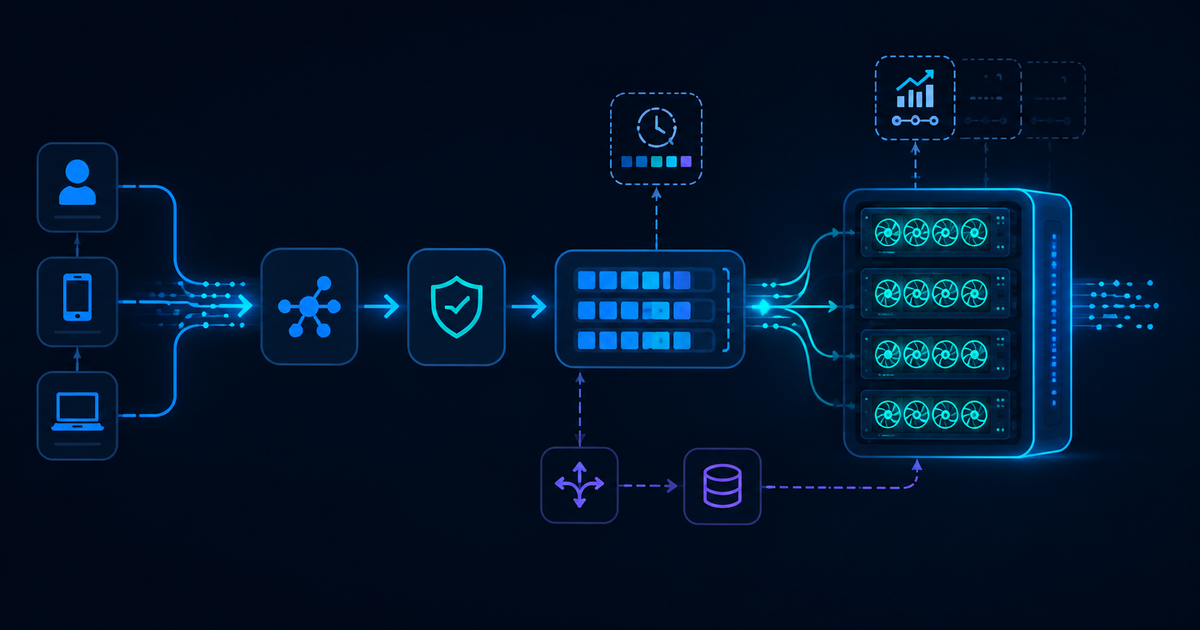
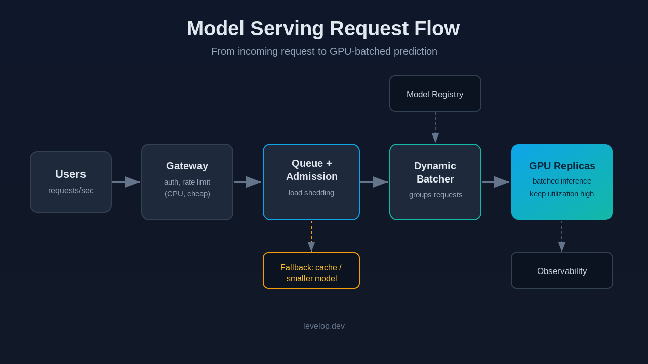
A production serving path is a small pipeline, and understanding the hops is the first step to reasoning about latency and failure. A request enters through a load balancer, hits an API gateway for auth and rate limiting, and lands on a serving replica. Inside the replica, a scheduler collects the input, groups it with other requests, runs the batch on an accelerator, and returns the result. A model registry tracks which model version to load, and an observability layer records latency, errors, and prediction distributions.

Separating these concerns matters because they scale differently. The gateway is CPU-bound and cheap to replicate. The model replica is GPU-bound and expensive. The cheap layer absorbs spikes and protects the expensive layer, which is the role a queue and an admission controller play in front of the accelerator. This layering is standard across a modern production environment.

Batching: The Biggest Lever You Have

GPUs are throughput machines and are inefficient at processing one request at a time, because a single input cannot saturate thousands of parallel cores. Batching, grouping several requests and running them through the model together, converts idle silicon into useful work. It is the most important optimization in model serving.

Static batching waits for a fixed number of requests or a fixed time window, then runs the whole batch. It is predictable but wastes time under light traffic. Dynamic batching adapts the window: it fires as soon as either a size threshold or a timeout is reached, so latency stays bounded under low load while throughput climbs under high load. For autoregressive large language models, continuous batching goes further, evicting completed sequences and admitting new ones token by token to keep the GPU near full utilization. This is why modern open source serving frameworks such as NVIDIA Triton Inference Server handle far more concurrent users than a naive one-request loop.

# Simplified dynamic batching loop for a serving replica
import asyncio, time

class DynamicBatcher:
    def __init__(self, model, max_batch=32, max_delay_ms=8):
        self.model = model
        self.max_batch = max_batch
        self.max_delay = max_delay_ms / 1000
        self.queue = asyncio.Queue()

    async def submit(self, x):
        fut = asyncio.get_event_loop().create_future()
        await self.queue.put((x, fut))
        return await fut

    async def run(self):
        while True:
            items, deadline = [], time.time() + self.max_delay
            while len(items) < self.max_batch and time.time() < deadline:
                try:
                    timeout = deadline - time.time()
                    items.append(await asyncio.wait_for(self.queue.get(), timeout))
                except asyncio.TimeoutError:
                    break
            if not items:
                continue
            xs = [x for x, _ in items]
            preds = self.model.predict_batch(xs)  # one GPU call for many inputs
            for (_, fut), p in zip(items, preds):
                fut.set_result(p)

The trade-off is latency variance. A larger maximum batch and longer window raise throughput but push out p99 latency for requests that arrive at the start of a window. Tune batch size and window against your latency budget, not against average latency.

GPU Management: Keeping Expensive Hardware Busy

GPUs are the largest line item in most model serving budgets, so utilization is the game. An accelerator sitting at 20 percent utilization wastes money. Model replicas should be sized so weights fit in GPU memory with headroom for activation memory that grows with batch size. Packing multiple small ai models onto one GPU, or using multi-instance GPU to partition a card into isolated slices, raises utilization when no single model needs the whole device. For very large models that do not fit on one GPU, tensor or pipeline parallelism splits the model across devices at the cost of coordination latency.

Autoscaling closes the loop between demand and capacity. Scaling on CPU is useless for GPU workloads; you scale on GPU utilization, queue depth, or batch latency. Because loading a large model into GPU memory takes tens of seconds, cold starts are a real design problem. Keeping a pool of warm replicas, and scaling ahead of demand using request-rate signals, keeps tail latency stable during ramps.

A/B Testing Models at Inference Time

Offline metrics are unreliable enough that you should not fully trust a new model until real traffic has seen it. Serving is where you learn whether the model that scored higher on validation actually helps users. The serving layer therefore needs first-class support for running several model deployments at once, each pinned to a specific model version.

The cleanest pattern is a routing layer that assigns each request to a variant using a stable hash of the user or session id. A stable hash keeps a user on the same variant across requests, which you need for a coherent experience and clean experiment analysis. You start a new model at a small traffic share, monitor models and business metrics, and ramp only if it holds. Shadow deployment is the safer cousin: you mirror live traffic to the new model but never return its output, so you can measure latency, error rate, and drift under production load with zero user risk before returning predictions to anyone.

# Stable-hash routing for inference-time A/B testing
import hashlib

def pick_variant(user_id: str, variants: dict) -> str:
    # variants: {"model_v3": 90, "model_v4": 10}  # percent of traffic
    h = int(hashlib.sha256(user_id.encode()).hexdigest(), 16) % 100
    cumulative = 0
    for name, pct in variants.items():
        cumulative += pct
        if h < cumulative:
            return name
    return next(iter(variants))

Graceful Degradation: Failing Without Falling Over

The hardest lesson in model serving is that the model will sometimes be unavailable, slow, or wrong, and the system still has to answer. Graceful degradation is the set of design choices that keep the product useful when the ideal path is broken. The first tool is the timeout and fallback chain: if the primary model does not respond within the latency budget, the request falls back to a smaller model, then to a cached result, then to a safe default. A recommender that cannot run its ranking model can still return popular items; search can fall back to keyword matching when the semantic model is down.

Load shedding protects the system under overload. When the queue in front of the GPU grows past a threshold, the admission controller rejects low-priority requests early, so high-priority traffic still meets its latency target. This is the serving version of a circuit breaker, described in the Google SRE book. Every degradation path must be observable: emit a metric on every fallback and cache hit, and alert when the fallback rate crosses a baseline. This is where model serving meets production observability, covered in our guide to LLM observability, and why the two are designed together.

Putting It Together

A production system for model serving in production is a layered design: a cheap front tier for auth and rate limiting, a queue and admission controller that protects the accelerators, GPU-bound replicas that use dynamic or continuous batching, a routing layer for A/B and shadow testing, and a fallback chain plus load shedding. None of these pieces is exotic. The skill is composing them against a latency, throughput, and cost budget, then measuring at the tail. Model serving is a systems problem in a machine learning costume: the levers, batching, utilization, safe rollout, and degradation, are the same distributed-systems levers engineers have used for decades. Explore more engineering guides at Levelop.