KV Cache and Continuous Batching: The Engine Behind Fast LLM Serving

If you have ever wondered why one LLM serving stack handles thousands of concurrent users on a handful of GPUs while another chokes on a few dozen, the answer usually comes down to two ideas: the KV cache and continuous batching. They are not glamorous. They rarely show up in model announcements. But they are the reason a well tuned inference server can push five to ten times more tokens through the same hardware.

This guide explains both mechanisms from first principles, shows how they fit together, and gives you the practical numbers to reason about throughput and memory on your own workloads. It is a companion to our LLM inference optimization developer's guide, which covers the full landscape. Here we go deep on the two techniques that do the heaviest lifting.

Why Naive LLM Serving Is So Slow

A transformer generates text one token at a time. To produce token number 100, the model attends over tokens 1 through 99. The obvious implementation recomputes the attention over the entire sequence at every step. That means generating an N token response costs work proportional to N squared, because step 1 processes 1 token, step 2 processes 2 tokens, and so on up to N.

For a 500 token answer that is roughly 125,000 units of attention work when it could have been 500. The recomputation is pure waste, because the model already computed the representations for every earlier token on the previous step. Nothing about those earlier tokens changed. This is the problem the KV cache solves.

The second problem is scheduling. Requests arrive at different times and finish at different times. A short reply might need 20 tokens, a long one 800. If you group requests into a fixed batch and wait for all of them to finish before starting the next batch, your fast requests sit idle waiting for the slow ones, and your GPU spends much of its time underutilized. This is the problem continuous batching solves.

What the KV Cache Actually Stores

Inside every attention layer, each token is projected into three vectors: a query (Q), a key (K), and a value (V). When the model generates a new token, its query vector attends over the keys and values of all previous tokens. The insight is simple. The keys and values for tokens already in the sequence never change as generation continues. So instead of recomputing them, you compute them once and store them.

That store is the KV cache. For each token, in each layer, you keep its key vector and its value vector. On the next generation step, the model computes Q, K, and V only for the single new token, appends the new K and V to the cache, and attends over the whole cache. The per step cost drops from quadratic to linear.

# Conceptual generation loop with a KV cache
kv_cache = None
tokens = prompt_tokens

for step in range(max_new_tokens):
    # Only the newest token is processed each step after the prompt
    logits, kv_cache = model(
        input_ids=tokens[-1:],   # single new token, not the full sequence
        past_key_values=kv_cache # keys/values for all prior tokens
    )
    next_token = sample(logits)
    tokens.append(next_token)
    if next_token == eos_id:
        break

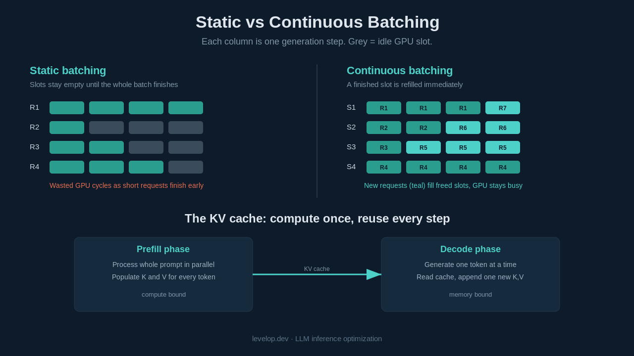
The generation of an LLM response splits cleanly into two phases because of this cache. The prefill phase processes the entire prompt in one parallel pass and populates the cache. The decode phase then generates output tokens one at a time, each step reading the growing cache and writing one new entry. Prefill is compute bound and highly parallel. Decode is memory bound and sequential, which is why decode throughput is so sensitive to how the cache is managed.

The Cache Is Not Free: Doing the Memory Math

The KV cache trades computation for memory, and that memory is substantial. You can estimate its size directly.

KV cache bytes = 2 * layers * num_kv_heads * head_dim
                 * sequence_length * batch_size * bytes_per_value

The leading factor of 2 accounts for storing both keys and values. Take a 13 billion parameter model with 40 layers, 40 attention heads, and a head dimension of 128, running in FP16 (2 bytes per value). For a single sequence of 2,000 tokens the cache is:

2 * 40 * 40 * 128 * 2000 * 1 * 2 bytes  =  about 3.3 GB

That is 3.3 GB of GPU memory for one request, on top of the model weights. Serve 20 such requests concurrently and the cache alone wants 66 GB. This is why KV cache memory, not raw compute, is usually the ceiling on how many requests you can batch together. Techniques like grouped query attention shrink the number of key value heads to cut this cost, and quantizing the model frees weight memory that the cache can then use.

PagedAttention: Fixing Cache Fragmentation

Early serving systems allocated KV cache in one contiguous block per request, sized for the maximum possible sequence length. If a request might generate up to 2,048 tokens, the server reserved space for 2,048 tokens even if the reply turned out to be 30 tokens long. The result was massive internal fragmentation. Studies of these systems found that only 20 to 40 percent of the reserved cache memory actually held useful data. The rest was reserved and wasted.

PagedAttention, introduced by the vLLM project, borrows the idea of virtual memory paging from operating systems. Instead of one big contiguous allocation, the cache is split into fixed size blocks, each holding the keys and values for a small number of tokens. A request is given blocks on demand as it generates, and a block table maps the logical sequence to the physical blocks wherever they live in memory. Nothing is reserved up front for tokens that may never be generated.

This near eliminates the fragmentation waste and lets the server pack far more sequences into the same GPU. It also unlocks memory sharing. Two requests with the same system prompt can point at the same physical blocks for that shared prefix, so the prompt is stored once rather than duplicated per request. That prefix sharing is closely related to semantic caching, though it operates at the token block level rather than the response level.

Continuous Batching: Keeping the GPU Busy

Now to the second engine. Batching many requests together is essential for GPU efficiency, because a GPU processing one sequence at a time leaves most of its parallel units idle. The naive approach, often called static batching, collects a fixed group of requests, runs them together until every one finishes, then starts the next group.

Static batching has a punishing flaw. Suppose a batch of eight requests includes seven that finish in 50 tokens and one that runs to 800 tokens. With static batching, the seven finished slots sit empty for the 750 extra steps while the last request grinds on. The GPU is holding a batch of eight but doing the useful work of one. Throughput collapses whenever response lengths vary, which in real traffic they always do.

Continuous batching, sometimes called in flight batching or iteration level scheduling, fixes this by making batching decisions at every generation step instead of every request. The scheduler runs the model one step, and as soon as any sequence emits its end of sequence token, that slot is freed. A waiting request is immediately slotted in to take its place. The batch is a living set that requests join and leave continuously.

Static batching (batch of 4):
  step ->  R1 R2 R3 R4
           R1 R2 -- R4      (R3 done, slot idle)
           R1 -- -- R4      (R2 done, slots idle)
           R1 -- -- --      (only R1 left, GPU mostly idle)

Continuous batching (batch of 4):
  step ->  R1 R2 R3 R4
           R1 R2 R5 R4      (R3 done -> R5 admitted immediately)
           R1 R6 R5 R4      (R2 done -> R6 admitted immediately)
           R7 R6 R5 R4      (R1 done -> R7 admitted immediately)

The difference in practice is dramatic. The original continuous batching research, the Orca system from 2022, reported throughput gains of more than an order of magnitude over static batching at similar latency, and production servers such as vLLM, NVIDIA TensorRT-LLM, and Hugging Face Text Generation Inference all build on the same idea today.

How the Two Mechanisms Depend on Each Other

KV cache and continuous batching are often described separately, but they only reach their full potential together. Continuous batching is what creates the demand for flexible memory. When requests join and leave the batch at arbitrary steps, you cannot know in advance how much cache each slot will need, so a rigid contiguous allocation would waste memory or fail outright. PagedAttention style block allocation is what makes the fluid membership of a continuous batch practical.

Run through the loop and the partnership is clear. The scheduler admits a new request, prefill runs and populates its cache blocks, decode steps generate tokens while the block table grows, and the moment the request finishes its blocks are returned to the pool for the next admission. The cache manager and the scheduler are two halves of one system. Weaken either and throughput drops.

Tuning Levers That Actually Move Throughput

Once you understand the machinery, the configuration knobs make sense. A few matter more than the rest.

The first is the fraction of GPU memory you allow the KV cache to occupy. Serving frameworks expose this directly, for example the gpu_memory_utilization setting in vLLM. Set it too low and you can batch fewer requests than the hardware could handle. Set it too high and you risk out of memory errors when long sequences arrive together. The right value depends on your model size and prompt distribution, and it is worth measuring rather than guessing.

The second is maximum batch size or maximum number of batched tokens. This caps how many sequences the scheduler admits. A larger cap raises peak throughput but also raises tail latency, because more sequences share each step. This is the classic throughput versus latency trade, and it ties directly into the cost and quality trade-offs of routing traffic across models.

The third is quantization of the KV cache itself. Storing keys and values in 8 bit or even 4 bit rather than 16 bit roughly halves or quarters cache memory, letting you batch proportionally more requests. The accuracy cost is usually small for well designed schemes, and the throughput gain is direct because cache memory is the binding constraint.

The fourth is chunked prefill, which interleaves the compute bound prefill of new requests with the memory bound decode of existing ones so a long prompt does not stall the whole batch. It smooths latency when prompts vary widely in length.

A Practical Serving Checklist

When you set up an LLM serving deployment, the following order of operations tends to give the best results. Choose a serving framework that implements paged KV cache and continuous batching rather than rolling your own, because the mature ones have spent years on edge cases. Size your GPU memory utilization by measuring, starting conservatively and raising it while watching for out of memory events under realistic load. Enable KV cache quantization if your accuracy budget allows, since it is the cheapest way to buy batch capacity. Benchmark with concurrent mixed length traffic, not single request loops, so your numbers reflect production. Finally, monitor cache utilization and preemption rates in production, because a rising preemption rate is the early signal that you are running out of cache memory and throughput is about to degrade. For the broader production picture, our model serving system design guide covers the surrounding architecture.

Where This Fits in the Bigger Optimization Picture

KV cache and continuous batching are foundational, but they are one layer of a stack. Above them sit techniques like speculative decoding, which reduces the number of expensive model steps, and model quantization, which shrinks the weights so more of the GPU is free for cache. These compose. A stack that pages its cache, batches continuously, quantizes both weights and cache, and speculatively decodes can serve an order of magnitude more traffic per dollar than a naive baseline. The full inference optimization guide walks through how to sequence them.

The reason to understand these two mechanisms specifically is that they set the ceiling. No amount of clever decoding helps if your cache fragments and your GPU idles between requests. Get the KV cache and the batching right first, and every other optimization has more room to work.

Want to go deeper on serving efficiency? Read the LLM inference optimization guide for the full stack, and browse more engineering write ups on the Levelop blog.